8 The bias-variance trade-off
In chapter 4, a decision tree’s max_depth lets more training accuracy come at the cost of worse test accuracy: too shallow, and the tree underfits; too deep, and it memorises (Figure 5.2). The same shape would appear for every model we’ve met since: \(k\) in KNeighborsClassifier, the regularisation strength on a linear model, etc. Training error keeps improving as complexity increases, while test error doesn’t. We’re going to analyse this behaviour.
8.1 Splitting the error into three pieces: bias-variance(-noise) decomposition
Suppose the data really is generated by some true function \(f\) plus noise:
\[y = f(x) + \varepsilon, \qquad \mathbb{E}[\varepsilon] = 0, \qquad \text{Var}(\varepsilon) = \sigma^2\]
We don’t know \(f\) or \(\sigma^2\); we only see a training sample and use it to fit an estimator \(g(x)\): a polynomial, a tree, a linear model, anything. Because \(g\) was fit on one particular training sample, a different sample would have given a different \(g\). So fix a point \(x_0\) and ask: averaged over all noise draws and all training samples we could have gotten, how far off is \(g(x_0)\) from a fresh \(y\) at \(x_0\)? That average is:
\[\mathbb{E}\big[(y - g(x_0))^2\big] = \underbrace{\sigma^2}_{\text{noise}} + \underbrace{\big(\mathbb{E}[g(x_0)] - f(x_0)\big)^2}_{\text{bias}^2} + \underbrace{\mathbb{E}\big[(g(x_0) - \mathbb{E}[g(x_0)])^2\big]}_{\text{variance}}\]
Each term answers a different question:
- Noise (\(\sigma^2\)): how much \(y\) itself jitters around \(f(x_0)\), regardless of any model. This is the part of the error no estimator can ever remove.
- Bias: how far the average fit, \(\mathbb{E}[g(x_0)]\) (averaged over all the training samples we could have drawn), sits from the truth \(f(x_0)\). A model that’s too simple to represent \(f\) at all has high bias, no matter how much data it sees.
- Variance: how much \(g(x_0)\) itself swings from one training sample to the next. A model flexible enough to chase the noise in whichever sample it happened to get will have high variance.
Both bias and variance depend only on \(g(x_0)\)’s behaviour across hypothetical training samples; neither depends on any one sample we actually have.
8.2 Synthetic simulation
The decomposition above is an average over all training samples we could have drawn. In practice we only ever get one. But in a simulation, we control the truth so that we can draw many samples, fit many models, and check the formula directly: generate \(M\) training sets of size \(N\) from a known \(f\), fit an estimator to each, and see how the \(M\) fits disagree with each other and with \(f\).
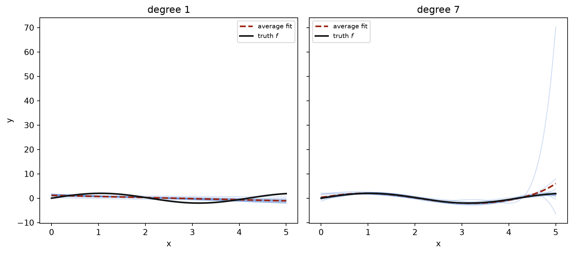
Here, \(f(x) = 2\sin(1.5x)\) on \([0, 5]\), with Gaussian noise added, \(N = 20\) points per training set, and polynomial regression (a linear model, applied to powers of \(x\)) as the estimator. The complexity is measured by the polynomial’s degree.
On the left, the degree-1 fits barely move from one training set to the next: that’s low variance. But a straight line cannot bend the way \(2\sin(1.5x)\) does, so even their average misses the shape: that’s high bias. On the right, the degree-7 fits bend enough to hug the curve, so their average tracks \(f\) closely: that’s low bias. But each fit is far away from the others: that’s high variance.
8.3 The trade-off, and where test error comes from
Because we simulated the data, we can also average many fits together to estimate the bias and variance themselves, at a grid of \(x\) points, for each degree:
\[\widehat{\mathbb{E}[g(x)]} = \frac{1}{M}\sum_{i=1}^M g_i(x) \qquad \widehat{\text{bias}}^2 = \Big(\widehat{\mathbb{E}[g(x)]} - f(x)\Big)^2 \qquad \widehat{\text{Var}} = \frac{1}{M}\sum_{i=1}^M \Big(g_i(x) - \widehat{\mathbb{E}[g(x)]}\Big)^2\]
Warning
With real data, we’re trying to estimate \(f\), and we only ever get the one training set we were given, never the \(M\) hypothetical ones needed to average over.
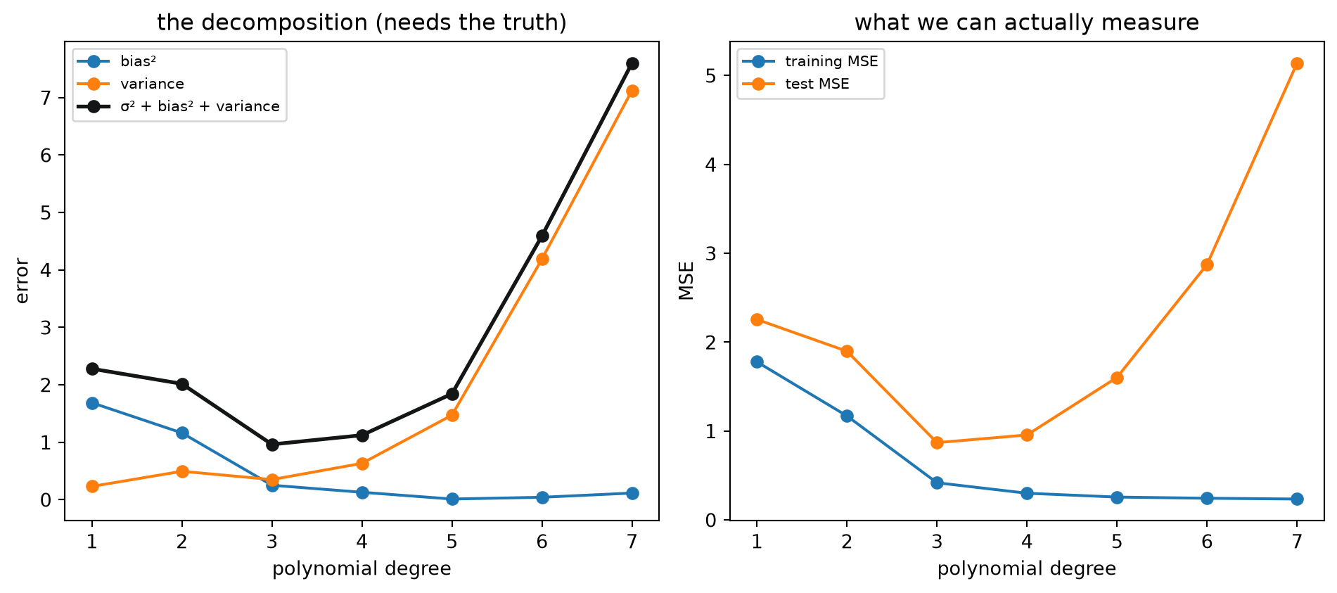
Both panels tell the same story from different vantage points. On the left, bias declines steadily as the polynomial gains flexibility to match the curve’s shape, while variance increases as each fit adapts to the sample’s noise; their sum, the total expected error, is U-shaped, with a minimum around degree 3. On the right (the quantities we could actually compute without knowing \(f\)), training MSE keeps falling as the degree grows, since a more flexible model always fits its own training points at least as well; test MSE is U-shaped, bottoming out at the same degree 3, then rising sharply as the high-variance, high-degree fits are increasingly wrong about data they weren’t fit on.
This is the bias-variance trade-off: pushing complexity up always buys lower bias, but never for free. Variance rises to pay for it. Too little complexity and the model can’t represent \(f\) no matter how much data it gets (underfitting, dominated by bias); too much and the model fits whichever noise its training sample happened to contain (overfitting, dominated by variance). The training-error curve alone cannot distinguish between the two, since it keeps improving in both regimes. That’s exactly why chapter 4 insisted on a held-out test set, or cross-validation, instead of trusting training performance.
NoteThe same shape, everywhere
Almost all models have a bias-variance trade-off:
| complexity measure | low value → | high value → |
|---|---|---|
| polynomial degree | high bias, low variance | low bias, high variance |
tree max_depth |
high bias, low variance | low bias, high variance |
\(k\) in KNeighborsClassifier |
low bias, high variance | high bias, low variance |
| regularisation strength | high bias, low variance | low bias, high variance |
Note \(k\) runs the other way: a small \(k\) averages over very few neighbours, so it tracks the training data closely (low bias, high variance), while a large \(k\) averages over many neighbours, smoothing out both the noise and the signal (high bias, low variance). For \(k\)-nearest-neighbour regression this can be made exact: at a point \(x_0\), with \(x_{(1)}, \dots, x_{(k)}\) its \(k\) nearest training points,
\[\mathbb{E}\big[(y - \hat{f}_k(x_0))^2\big] = \sigma^2 + \Big(f(x_0) - \frac{1}{k}\sum_{\ell=1}^k f(x_{(\ell)})\Big)^2 + \frac{\sigma^2}{k}\]
the variance term shrinks with \(k\) as \(\sigma^2/k\), exactly like the variance of any average of \(k\) numbers; the bias term grows with \(k\) because the \(k\)-th neighbour is, on average, farther from \(x_0\) as \(k\) grows (Hastie et al. 2009).
8.4 Getting both down at once
Variance also shrinks with more training data: more points pin a flexible model down to the true shape, since any one sample’s noise gets outweighed by the rest. Bias, by contrast, is fixed by the model’s hypothesis class, not its sample size. A straight line stays a straight line no matter how many points it’s fit to. More data alone never fixes an underfitting model; it only tames overfitting.
Restricting the hypothesis class, assuming that the true function has a certain form before seeing any data, is called the model’s inductive bias. Adding this bias only makes sense if it lowers the variance.
There’s a second route to lower variance without changing the degree at all: fit many flexible (hence high-variance, low-bias) models and average their predictions. Averaging \(M\) independent fits divides their variance by roughly \(M\), the same arithmetic as the \(\sigma^2/k\) term above, while leaving bias essentially untouched. A flexible model is still a good match for \(f\) on average. We’ll put this to work directly when we encounter ensemble methods, such as random forests, later in the course.