flowchart LR
    x(("x")) --> nature("nature") --> y(("y"))
1 Why study machine learning?
Assume you have
- a question about the world (or nature or life),
- data.
We’ll treat nature as a black box which associates an input variable \(x\) with an output variable \(y\):
Think of \(x\) and \(y\) as very long vectors (lists of numbers) that represent a particular state of the world (or the part you’re focusing on). In statistical terms, \(x\) is the predictor variable and \(y\) is the response variable.
Machine Learning is a set of techniques to approximate the black-box mapping between \(x\) and \(y\). More precisely, ML builds models from so-called training data that generalize well to new, unseen observations. Importantly, in ML, there’s a great emphasis on the computational side of things, because models can be complex and prediction is made on many data points.
There is the astonishingly wide range of applications, in terms of
- fields, e.g. biology, psychology, physics, (all experimental sciences, you name it!), business and politics (hopefully!),
- objectives,
- quality/quantity of data,
- etc.
1.1 Two motivating examples
To make this concrete, let’s look at two running examples.
Find a penguin’s species from its measurements. Given a penguin’s bill length, bill depth, flipper length, and body mass, can we tell whether it’s an Adelie, Chinstrap, or Gentoo penguin?
| species | island | bill_length_mm | bill_depth_mm | flipper_length_mm | body_mass_g | sex | |
|---|---|---|---|---|---|---|---|
| 0 | Adelie | Torgersen | 39.1 | 18.7 | 181 | 3750 | MALE |
| 1 | Adelie | Torgersen | 39.5 | 17.4 | 186 | 3800 | FEMALE |
| 2 | Adelie | Torgersen | 40.3 | 18.0 | 195 | 3250 | FEMALE |
| 3 | Adelie | Torgersen | 36.7 | 19.3 | 193 | 3450 | FEMALE |
| 4 | Adelie | Torgersen | 39.3 | 20.6 | 190 | 3650 | MALE |
Here, \(y\) (the species) is discrete: it takes one of a handful of category labels.
Predict a person’s income. Given someone’s age, marital status, education, hours worked per week, workclass, and so on, can we predict their income?
| age | workclass | fnlwgt | education | educational-num | marital-status | occupation | relationship | race | gender | capital-gain | capital-loss | hours-per-week | native-country | |
|---|---|---|---|---|---|---|---|---|---|---|---|---|---|---|
| 0 | 39 | Self-emp-not-inc | 327120 | HS-grad | 9 | Married-civ-spouse | Craft-repair | Husband | White | Male | 0 | 0 | 40 | Portugal |
| 1 | 32 | Private | 123253 | Assoc-acdm | 12 | Married-civ-spouse | Craft-repair | Husband | White | Male | 0 | 0 | 42 | United-States |
| 2 | 47 | Private | 232628 | HS-grad | 9 | Married-civ-spouse | Craft-repair | Husband | Black | Male | 0 | 0 | 40 | United-States |
| 3 | 19 | Private | 374262 | 12th | 8 | Never-married | Handlers-cleaners | Own-child | White | Male | 0 | 0 | 20 | United-States |
| 4 | 46 | Self-emp-not-inc | 311231 | HS-grad | 9 | Married-civ-spouse | Farming-fishing | Husband | White | Male | 0 | 0 | 40 | United-States |
Here, \(y\) (the income) is continuous: it’s a numerical quantity.
These two examples illustrate the two main flavours of the prediction problem, which we’ll define precisely below.
Engineering rules versus data-driven rules. One way to build a predictive rule is to rely on expert knowledge. For instance, an ornithologist might tell us: Adélie penguins have shorter bills (shorter culmen) than Chinstrap or Gentoo penguins.
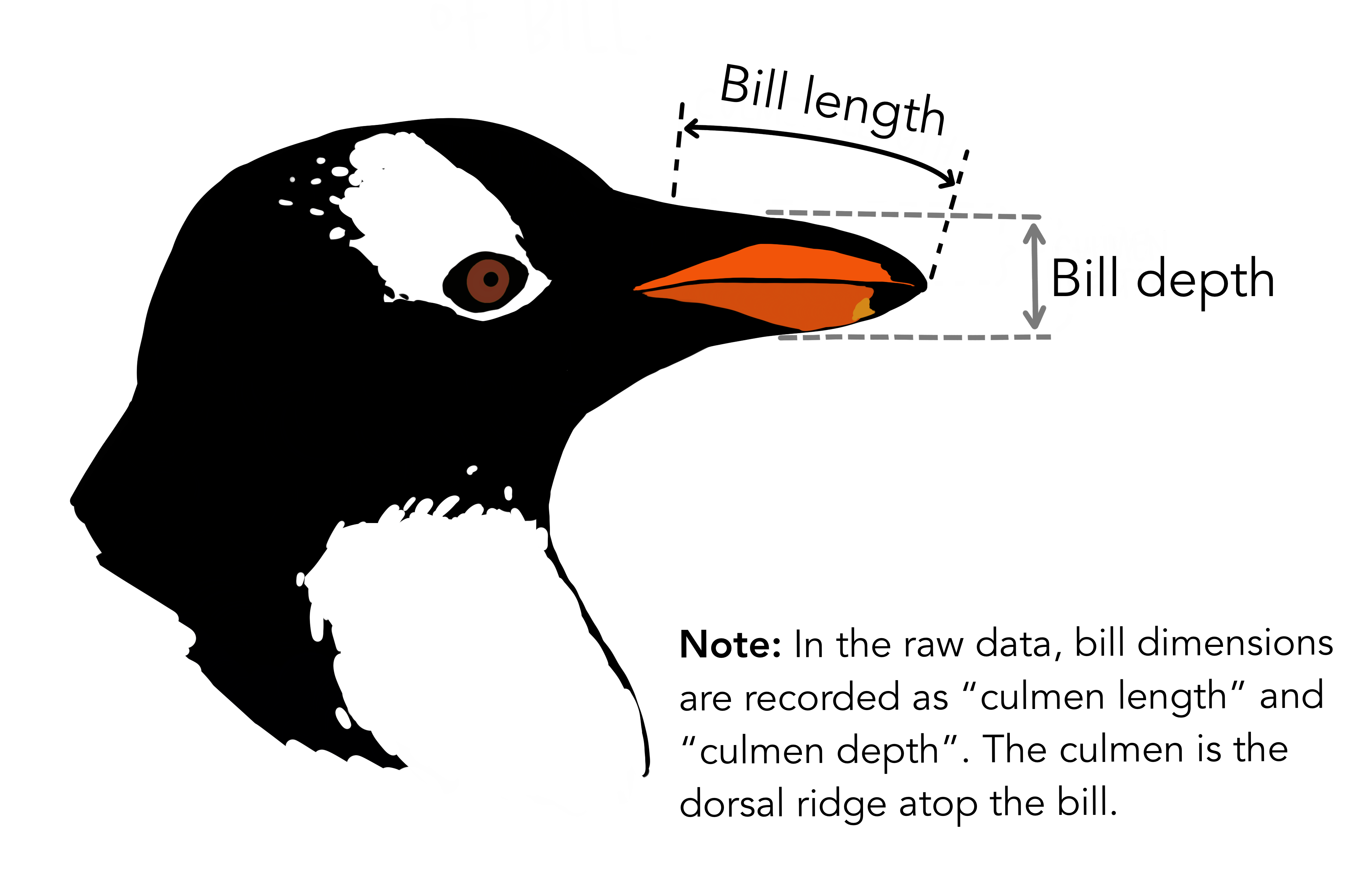
The appeal of machine learning is that this same rule can often be inferred directly from the data, without an expert having to state it explicitly:
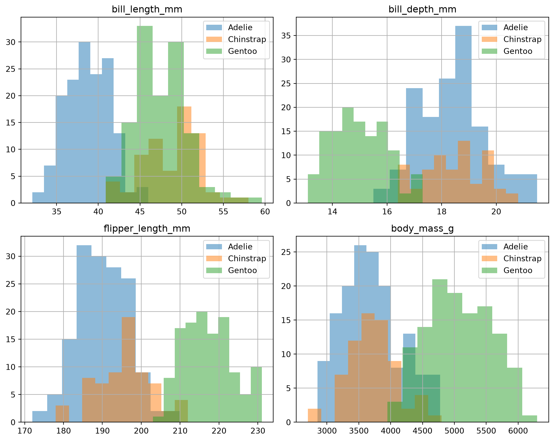
Plotting the distribution of each measurement by species shows visually that some features (like bill length) separate the species quite well. An ML model could pick this up on its own.
This is what makes machine learning attractive: it goes beyond classic statistical tools by letting the data itself surface predictive rules that would otherwise require a domain expert.
1.2 A few key terms
The data matrix. To fit these models, we organize our data into a table (figuratively, a spreadsheet):
- rows are different observations, or samples;
- columns are different descriptors, or features.
We call X the data matrix of features, and y the vector of labels (the target variable we want to predict). X has shape n_samples x n_features, and y has length n_samples.
Supervised learning starts from a data matrix X with n observations and a target y: a property of each observation that we want to predict from the features. The objective is to predict the target y (e.g. species) from the features X (e.g. measurements).
Within supervised learning, we distinguish two problem types by the nature of y:
- Classification:
yis discrete (qualitative), made of different classes, e.g. Adelie, Gentoo, Chinstrap. - Regression:
yis continuous (quantitative), a numerical quantity, e.g. income.
Unsupervised learning, by contrast, only has a data matrix X and no target y. The goal, instead, is to extract a generalising structure from X. This covers a very wide variety of problems, which we’ll only touch on later in the course.
WarningGeneralizing \(\neq\) memorizing
Consider the simplest possible model: “nearest neighbours”. Store every observation we’ve ever seen, and when given a new one, predict using its closest match in that stored database.
If we evaluate this strategy on the very individuals it memorised, the error rate is zero by construction. But on genuinely new data, we should expect errors: new individuals differ in their sampling of noise, and may present combinations of features we’ve never observed before.
This is why machine learning always separates data into (at least) two parts:
- Train data: used by the model to “learn” its rules.
- Test data: held out, and used only to check how well the model performs on observations it did not memorise.
A model that merely memorises its training data (like the nearest-neighbours strategy above, taken to the extreme) tells us little about how it will behave on new data. What we actually care about is generalisation: performing well on the test set, not just the training set.
1.3 How to decompose ML methods
Here, we focus on supervised methods. To understand a new ML procedure, a good starting point is to determine the following elements.
- The predictor: the input variable, always observed.
- The response: the output variable, not observed except, sometimes, on a set of examples (see training data).
- Model: the function mapping input to output.
- Training data: a set of example pairs (predictor, response) used to calibrate and compare different models.
- Error metric: a measure of whether a prediction is close to the ground truth (provided in the training data) or not.
- The learning procedure: the procedure used to find the model parameters that minimise the error metric on the training data.
Side note: The model need not be close to the true underlying data-generating mechanism, as long as it has good predictive power.
1.4 “Can’t I just AI?”
This question is haunting many students’ minds, for good reasons. However, LLMs can’t replace well-trained analysts just yet. LMMs will be of tremendous help when it comes to coding, but they still leave a lot of conceptual errors, that can only be corrected by ML specialists. I expect that bugs in data processing pipelines to be conceptual rather than simple code mistakes. A proper education in ML will be key to create efficient ML pipelines.
Also, there is a good chance that tokens will become less and less affordable. Driving LLMs towards the correct solution with relevant feedback prompts will certainly set you apart.
NoteIn-class activity
You don’t have to take my word for it. Let try to build a resume screening algorithm using an LLM.
I’ll then show you how a trained ML analysts might build it, using the correct tools and providing helpful feedback.
1.5 References
Al Mamun, Md. Abdullah, Mou Rani Sarker, Md Abdur Rouf Sarkar, et al.
2024. “Identification of Influential Weather Parameters and
Seasonal Drought Prediction in Bangladesh Using Machine Learning
Algorithm.” Scientific Reports 14 (1). https://doi.org/10.1038/s41598-023-51111-2.
Brilliantina, Aulia, Tri Agus Siswoyo, Yuli Witono, and Bayu Taruna
Widjaja Putra. 2026. “Development of Non-Destructive Durian Fruit
Maturity Detection Tool Based on Multi-Variable Sensor for Harvest
Quality Optimisation.” Scientific Reports, ahead of
print. https://doi.org/10.1038/s41598-026-61395-9.
Hastie, Trevor, Robert Tibshirani, and Jerome Friedman. 2009. The
Elements of Statistical Learning: Data Mining, Inference, and
Prediction. 2nd ed. Springer Series in Statistics. Springer. https://hastie.su.domains/ElemStatLearn/.
Horst, Allison Marie, Alison Presmanes Hill, and Kristen B Gorman. 2020.
Palmerpenguins: Palmer Archipelago (Antarctica) Penguin Data.
https://doi.org/10.5281/zenodo.3960218.
Natarajan, Suresh Kumar, Prakash Shanmurthy, Daniel Arockiam,
Balamurugan Balusamy, and Shitharth Selvarajan. 2024. “Optimized
Machine Learning Model for Air Quality Index Prediction in Major Cities
in India.” Scientific Reports 14 (1). https://doi.org/10.1038/s41598-024-54807-1.